Demand during the Risk Period
This page provides a summary of problems discussed in the book
Under conditions of uncertainty the demand during the risk period plays a central role. The risk period is composed of
- the review period and
- replenishment lead time.
Stochastic demand occurs within this time span that usually comprises several periods. In order to compute the parameters of an inventory policy, we must know the probability distribution of the demand during the risk period. In the sequel we assume that the considered standard period length is one day. The period demands $D$ for the focused product are random variables which are uncorrelated over time and which have a stationary probability distribution (e.g. normal distribution, gamma distribution, discrete empirical distribution.). In cases with dynamic period demand which changes its level over time, demand over the risk period is forecasted. The forecast error is the random variable that must be accounted for with the help of safety inventory. Assume that the probability distribution of the period demand has been estimated based on dataobserved in the past. The systematical monitoring of the development of the demand is an often neglected, but absolutely essential, prerequisite for the application of an inventory policy under stochastic conditions.
In case of a continuous representation, the period demands $D$ are described by a density function $f_{D}(d)$ and a probability distribution function $F_{D}(d)=P\{D\le d\}$. If demands are discrete, the probabilities $P\{D=d, d=d_{\mathrm{min} },\ldots,d_{\mathrm{max} }\}$ are given.
The lead time $L$ may be modeled as a random variable, too. If this option is considered, we assume that $L$ follows a discrete probability distribution $P\{L=\ell, \ell=\ell_{\mathrm{min} },\ldots,\ell_{\mathrm{max} }\}$. This modeling of the time axis with discrete time buckets is in accordance with the usual order of events which is observed in logistical processes. For example, if a replenishment order is sent to a supplier, say, at 2.30pm, then even under advantageous conditions (order transfer via Internet, supplier has stock on hand, etc.) the order will arrive the following morning at the earliest. Continuous replenishment lead times that can be modeled with the help of a continuous, i.e. exponential, probability distribution are quite rare in industrial practice.
Deterministic lead times
With a given value $\ell$ of the replenishment lead time, the demand during lead time, $Y$, is the sum of $\ell$ period demands. The probability distribution of this sum depends on the probability distribution of the period demands. In industrial practice many different types of demand distributions are observed. For slow-moving products the Poisson distribution may be appropriate. In other cases the gamma distribution provides a flexible means for modeling the randomness of the period demands. In the following we use the normal distribution, the gamma distribution, and a discrete empirical probability distribution to model period demands.
Normal distribution. If the period demands $D$ follow a normal distribution with mean $\mu_{D}$ and standard deviation $\sigma_{D}$, then the demand during the deterministic lead time $\ell$ is also normal distributed with mean $\mu_{Y} = \mu_{D} \cdot \ell$ and standard deviation $\sigma_{Y} = \sigma_{D}\cdot \sqrt{\ell}$.
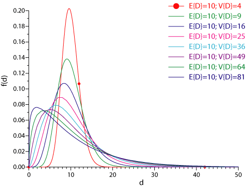
Gamma distribution. If the period demands $D$ follow a gamma distribution with scale parameter $\alpha_{D}$ and shape parameter $k_{D}$, then the demand during $\ell$ periods is also gamma distributed with scale parameter $\alpha_{Y}=\alpha_{D}$ and shape parameter $k_{Y}=k_{D}\cdot \ell$. The following Figure shows the density functions of gamma distributions with different coefficients of variation $\mathrm{CV}\{D\}=\frac{\sqrt{Var\{D\}}}{E\{D\}}$. Observe that fairly different shapes of demand structures can be modeled with the help of the gamma distribution.

Discrete empirical distribution. If the period demand is distributed according to an empirically observed discrete probability distribution, then the probability distribution of the demand within $\ell$ periods can be computed through the $\ell$-fold convolution of the single-period probability distribution as follows. Let $Y^{(\ell)}$ be the sum of the demands of $\ell$ period, then we have:
$P\left\{ {Y^{(1)}=y_k} \right\}=P\left\{ {D=y_k} \right\}$
and
$P\left\{ {Y^{(\ell)}=y_k}
\right\}=\displaystyle{\sum_{x_i+d_j=y_k}} {P\left\{ {Y^{{(\ell-1)}}=x_i,D=d_j}
\right\}} \qquad \ell\ge2$
More details are provided in the book
Random lead times
In practice lead times are usually random because the replenishment lead time observed by the customer is the customer order waiting time from the point of view of the supplier. It is well-known that the customer order waiting times are random, if
- the supplier produces to order (make-to-order, MTO) and random flow times (caused by machine breakdowns, scrap, etc.) or non-controllable flow times occur during the production processes. One reason for this may be the application of inadequate planning procedures for production planning, e. g. lotsizing based on the unrealistic assumption of infinite capacities as performed in MRP planning systems.
- the supplier produces to stock (make-to-stock,MTS), but is not able to guarantee a 100% service level. Note that the replenishment lead time (of the customer) depends on the inventory policy applied by the supplier. For example, if the supplier uses a (r, S) policy, then the risk of long customer waiting times is larger than with an equivalent (s, q) policy.
- additional logistic processes with random duration, such as order processing and handling or transportation have to be run through. This is usually the case in industrial practice.
- the planning system of the customer uses a time axis with shorter time periods than the order processing system of the supplier (e. g. if the supplier has a weekly delivery cycle and the customer reviews his inventory position on a daily basis). In this case the customer may react in time on the development of his inventory position. But this timely reaction does not give him any advantage, as he has to wait until the supplier starts his order processing at the beginning of the next period. In this case, the replenishment lead time of the customer depends on the (residual) waiting time for the next order processing by the supplier, with the result of more or less long (random) replenishment lead times.
A popular proposal to account for stochastic replenishment lead times is as follows. It is assumed that the lead times are stationary random variables with expected value $E\{L\}$ and variance $Var\{L\}$ and that they are independent from the size of the period demands. Note that from lotsizing models we know that this will usually not be true, as under binding capacity constraints the service time of a production facility depends on its utilization. The demand during lead time, $Y$, is then the sum of a random number of random variables. The expected value of $Y$ is
$E\left\{ Y \right\}=E\left\{ L \right\}\cdot E\left\{ D \right\}$
For a given value of the replenishment lead time, $L=\ell$, we use the
equivalence $Var\{X\}=E\{X^2\}-E\{X\}^2$ yielding
$Var\{Y|L=\ell\}=E\{Y^{2}|L=\ell\}-(\ell\cdot E\{D\})^2$
or
$E\{Y^{2}|L=\ell\}=\ell\cdot Var\{D\}+(\ell\cdot E\{D\})^2$
If $L$ is random, we obtain
$Var\{Y\} ={\sum_{\ell} \big[ \ell \cdot Var\{D\}+(\ell\cdot E\{D\})^2\big]} \cdot P\{L=\ell\} - {E\{D\}^2\cdot E\{L\}^2} $
More details are provided in the book
The variance of the demand during the lead time is therefore
$Var\left\{ Y \right\}=E\left\{ L \right\}\cdot Var\left\{ D \right\}+Var\left\{ L \right\}\cdot E\left\{ D \right\}^2$
Examples are provided in the book
The influence of the form of the probability distribution of the replenishment lead time on the probability distribution of the demand during the risk period
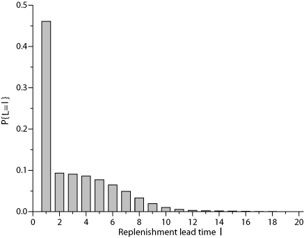
The form of the probability distribution of the demand during the risk period $Y$ is influenced, among others, by the form of the probability distribution of the replenishment lead times, whereby in many cases multi-modal densities of the demand during the risk period far from the normal density may result. Consider the frequency distribution of the lead time presented in the following Figure, which was observed in a simulation study (see also Examples for waiting time distributions under an ($r,s,q$) Policy in discrete time). This distribution is typical for a supplier who runs an inventory system in order to serve his customers and who achieves only a low service level.

A situation like this is likely to be observed in multi-level supply chains, when the supplying node as well as the customer node are owned by the same company and are optimized simultaneously. In this case it may, from a system-wide perspective, be optimal to hold only a very small safety stock in the supplying node which leads to poor delivery performance and long waiting times for replenishment in the customer node.(see also The role of the waiting time distribution in a multi-level inventory system).
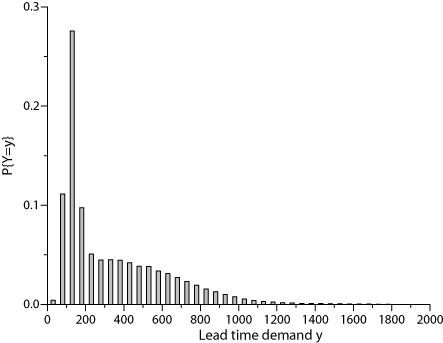
Now, assume that the period demand is normally distributed with mean $\mu=100$ and standard deviation $\sigma=30$. Then, for the depicted lead time distribution we get the following probability distribution of the demand during the lead time. Then, according to the relations mentioned above, for the depicted lead time distribution (with $E\{L\}=3.12$, $Var\{L\}=7.28$) we get a lead time demand with expectation $E\{Y\}=312$ and variance $Var\{Y\}=75617$ (standard deviation 275). The coefficient of variation for this probability distribution is $\mathrm{CV}_Y=0.88$.

A short look at the Figure reveals that this distribution is not a normal distribution. Nevertheless, in industrial practice in most cases the normal distribution is assumed. This may lead to significant deviations from optimality. This problem is discussed in an increasing number of publications.
Many vendors of inventory management software (and also their customers) do not take notice of these problems. The following example demonstrates the penalty costs that can arise from the wrong approximation of the lead time demand. Assume that in an inventory node a $(r,S)$ policy with $r=10$ and a target service level $\beta=0.95$ is in effect. The correctly computed value of the order level is in this case $S=1505$. Approximating the lead time demand $Y$ with a normal distribution with parameters $\mu_Y=312$ and $\sigma_Y=275$ would yield $S=3971$ which is by far too much.
More details are found in the book.